Finding the Alpha or Beta in Data.

As my Data Science journey has continued in these past few weeks, I’ve learned to extract clean information from raw data to form actionable insights. This has aided in my understanding of LINEAR AND MULTIPLE LINEAR regression, machine learning fundamentals and really caused my curiosity to pique. While continuing to learn daily, my knowledge and confidence has been growing exponentially. I am feeling more driven than ever to start applying what I am learning.

Today I will share a tutorial of Simple Regression Technique in Python.

We’re going to be taking a look at a simple regression technique in Python. There are a plethora of tools available to implement regression in Python. We are going to look at a couple of them, specifically, what you can do with Numpy. It is not meant to be an exhaustive tutorial on all the methods of regression in Python and we’re not going to be running any statistical tests. We are just going to be fitting a line and then visualizing the output of that fit line.

The first step is to import these libraries. Libraries are a Data Scientist’s best friend. In Data Science, there is always a lot of action going on behind the scenes. At first glance they look like words, but behind every “Import” there are a wealth of features that can help you in your coding and your project.

import numpy as np
import pandas as pd
import pandas_datareader as pdr
import matplotlib.pyplot as plt
import seaborn as sb
sb.set()
import datetime as dt
from datetime import date
import requests
from bs4 import BeautifulSoup as soup

Get data for SPY and GOOG

Next we’re going to go out and gather our data. Data for Google and the S&P 500 etf . We’ll go back about a year okay(365) and then we’ll store our data using the pandas datareader and the Yahoo Finance API.

stocks = "GOOG SPY".split()
start = dt.date.today() - dt.timedelta(365)

We then create another variable named “data”.

data = pdr.get_data_yahoo(stocks, start)
data.head()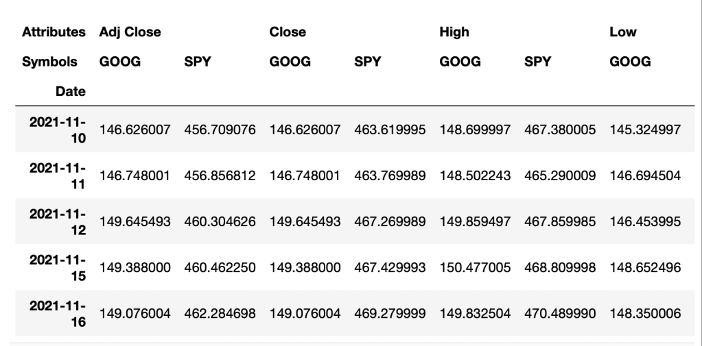

By adding (.head) this will show you the first few lines of your dataset. We actually don’t need all of this data, so you can see we get a high low open close and an adjusted close and volume. All you really need is the close for what we’re going to be doing, so I’m going to go back and adjust the data by adding [“Close”] to the data set below:

data = pdr.get_data_yahoo(stocks, start)["Close"]
data.head()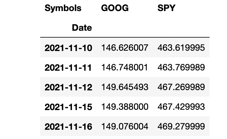

We’re not going to be using the closing prices directly, so I’m going to calculate the instantaneous rate of returns for both Google and the S&P 500 etf.

returns = np.log(data).diff()
returns.head()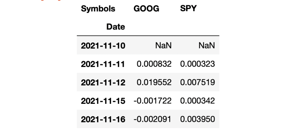

I notice the first value can not be calculated so I will drop that nan by adding “.dropna()”. You can either re-type or copy from the cell above.

returns = (np.log(data).diff()).dropna()
returns.head()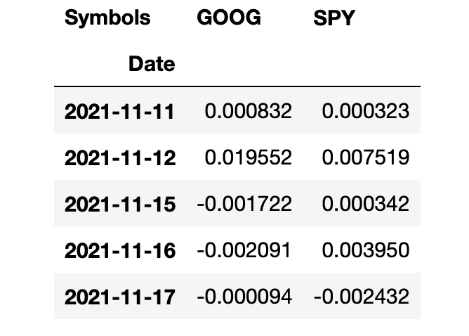

With all that, we are now ready to sort of start looking at a regression. I think the first thing that makes sense to do is probably get a correlation here. So I will take our returns and I’m going to apply the pandas method (.corr) and we can see they’re pretty strongly correlated.

sample= returns.sample(60).corr()
sample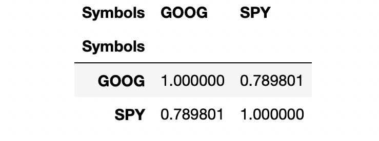

Since the S&P 500 is a market cap weighted index and Google happens to be very large, it’s a question if we’re running a regression here to calculate a beta or something like that. So, the question here is, is Google causing the S&P 500 to go up or is S&P 500 causing Google to go up? We’re not going to try to answer that question. We’re just going to go ahead and put S&P 500 as the independent variable here.

#Its probably better to get a smaller sample so you can have better visibility so I will be sampling this data to 60 returns
#X=being the predictor or independent variable and  
#Y=the dependent variable and Voila! There is our scatter plot
sample = returns.sample(60)
plt.scatter(x=sample['SPY'], y=sample['GOOG']);

View Preview

So now I’m going to set a variable and call it “reg” and I’m going to use the Numpy polyfit.

So we get the “Slope” and “Y” intercept there. So it looks like for every 1.18% the S&P 500 goes up, you can expect GOOG to go down slightly .003 % and this would be equivalent to what we predict as -Beta. It’s unusual for stocks to have a negative Beta. However, a stock with a Beta >1 would mean a volatile stock, and a Beta <1 means it’s less volatile.

Now we can go ahead and plot the scatter plot and plot the trend line. There is our best fit line graphed against the sample
of data points that we chose from above.

trend = np.polyval(reg, sample['SPY'])
plt.scatter(sample['SPY'], sample['GOOG'])
plt.plot(sample["SPY"], trend, 'r');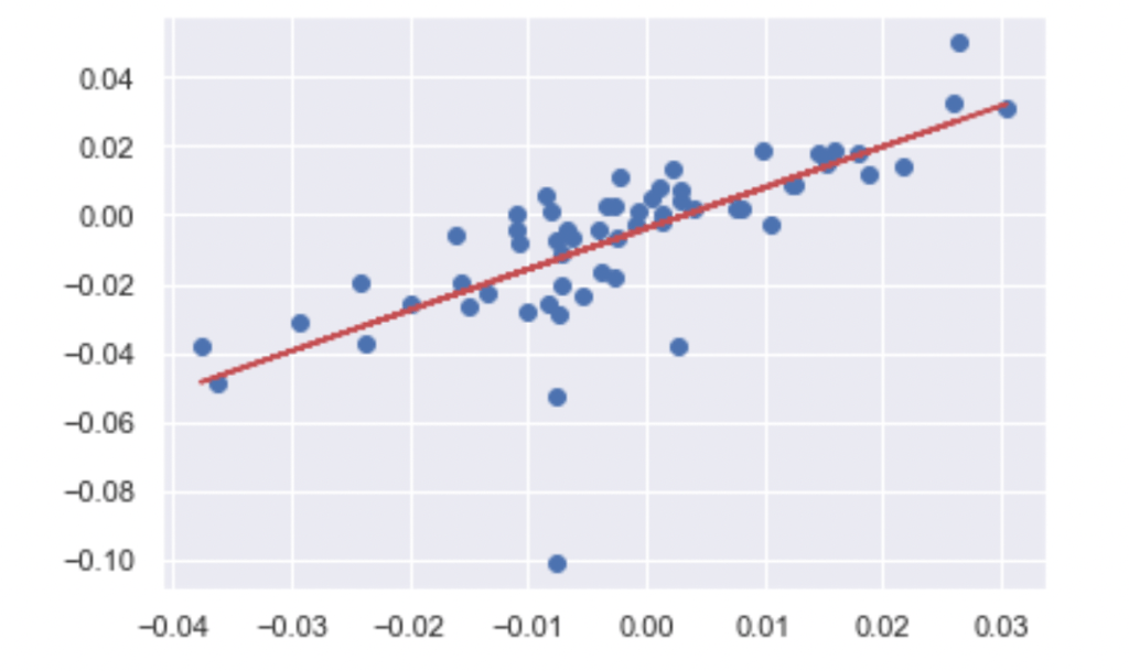

Hopefully, this short tutorial piques your curiosity about what you can learn in Data Science.